Wind speed and direction tutorial

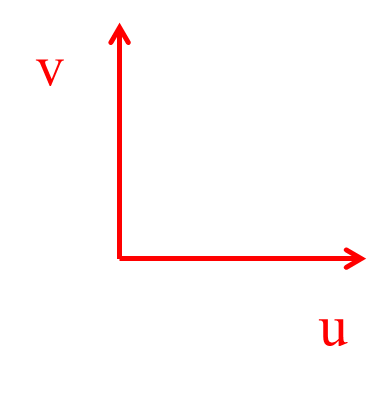
Originally, climate reanalysis data provide wind speed separately for Eastward (u) and Northward (v) directions. These are two different vectors.

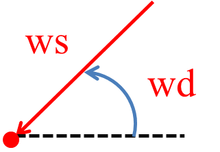
However, for most applications it is preferably to have wind speed (ws) and wind direction (wd) (azimuth) values instead.

This tutotial shows how to convert u-v vectors to wind speed and direction using RWikience. Wind speed and direction data exploratory tools are also introduced.

Prerequisite: you should have RWikience installed into R.
This RWikience introductory tutorial is also worth seeing.

Launch Climate Wikience. RWikience will be able to retrieve data only if Climate Wikience is currently running on your desktop.

Start your work by loading RWikience package and connecting to running Climate Wikience from R. Note: Climate Wikience should be running for successful connection.

# Load RWikience package
library(RWikience)
 
# Connect to Climate Wikience 
w<-WikienceConnect()

Time series retrieval consists of two parts.

1. Call “queryTimeSeries” with necessary parameters to prepare time series
2. Call other functions (find out number of points, retrieve time series for a selected point and other functions) to work with prepared time series

The next code retrieves (prepares) time series for

• Eastward wind speed at 10 meters altitude
• for each point in geographical region where
  • latitude south = -25,
  • longitude west = 130,
  • latitude north = -24,
  • longitude east = 131
• and time interval spans
  • since 1-st of January 1979 (inclusively)
  • to the 1-st of August 2014 (exclusively)

queryTimeSeries(w, "MERRA.Wind.Eastward (u).10 m", "01 01 1979", "01 08 2014", -25, 130, -24, 131)

NOTE: there are no limitations on time interval maximum length when you retrive time series using R unlike requesting time series in Climate Wikience.

You can copy/paste dataset name (i.e. MERRA.Wind.Eastward (u).10 m) from Climate Wikience (select the dataset in the tree on “Temporal layers” tab, the dataset name will appear in “Time Slider” drop-down list or “Properties” drop-down list)

Once the preparing operation finishes, you can check the number of points in the result (the output should be 6)

getTimeSeriesPointCount(w)

The coordinates of the resulting 6 points could be seen by calling

latlon <- getTimeSeriesPointsLatsLons(w)
latlon

The output should look like this:

lat      lon
1 -25.0 130.0000
2 -25.0 130.6667
3 -24.5 130.0000
4 -24.5 130.6667
5 -24.0 130.0000
6 -24.0 130.6667

Let’s take the first point in the result (it has coordinates lat = -25.0, lon = 130.0 ). Since data is hourly, there are 311904 values for the selected time interval

tU <- getTimeSeries(w, 0)
 
# See the first 10 values
tU[1:10,]
                  date     value
1  1979-01-01 00:00:00 -5.768760
2  1979-01-01 01:00:00 -4.866543
3  1979-01-01 02:00:00 -4.114307
4  1979-01-01 03:00:00 -3.606280
5  1979-01-01 04:00:00 -3.326102
6  1979-01-01 05:00:00 -3.213083
7  1979-01-01 06:00:00 -3.231349
8  1979-01-01 07:00:00 -3.344310
9  1979-01-01 08:00:00 -3.563092
10 1979-01-01 09:00:00 -3.926733

In this tutorial we will concentrate on the single location (point). We have u-vectors (tU) for this single point and now we will retrieve v-vectors (Northward wind speed component) for the same time interval and geographical region

queryTimeSeries(w, "MERRA.Wind.Northward (v).10 m", "01 01 1979", "01 08 2014", -25, 130, -24, 131)

Since query parameters are the same, the result contains time series for the same points. Thus, the first point will also have coordinates lat = -25.0, lon = 130.0. Now, get this first point from the result:

tV <- getTimeSeries(w, 0)
 
# Again, the first 10 rows are
tV[1:10, ]
                  date      value
1  1979-01-01 00:00:00 -1.2735988
2  1979-01-01 01:00:00 -1.2039323
3  1979-01-01 02:00:00 -0.8677690
4  1979-01-01 03:00:00 -0.5525676
5  1979-01-01 04:00:00 -0.2276626
6  1979-01-01 05:00:00  0.1847073
7  1979-01-01 06:00:00  0.6056390
8  1979-01-01 07:00:00  0.9443905
9  1979-01-01 08:00:00  1.1709728
10 1979-01-01 09:00:00  1.1513032

Now we have both u and v vectors for the point. Call the “convertUVtoSpeedAndDirection” function from RWikience package to obtain the data frame containing date, wind speed (ws) and wind direction (wd) columns.

Note: wind speed and direction values comply with the UK meteorological office standards. Wind direction is the azimuth (where FROM does the wind blow) as shown on the figure at the top of this tutorial (ws and wd).

result <- convertUVtoSpeedAndDirection(tU, tV)
 
# Check the first 10 rows
result[1:10, ]
                  date       ws        wd
1  1979-01-01 00:00:00 5.907677  77.55023
2  1979-01-01 01:00:00 5.013252  76.10461
3  1979-01-01 02:00:00 4.204824  78.09002
4  1979-01-01 03:00:00 3.648367  81.28868
5  1979-01-01 04:00:00 3.333884  86.08437
6  1979-01-01 05:00:00 3.218388  93.29008
7  1979-01-01 06:00:00 3.287615 100.61556
8  1979-01-01 07:00:00 3.475095 105.76900
9  1979-01-01 08:00:00 3.750574 108.19257
10 1979-01-01 09:00:00 4.092033 106.34094

The next section of the tutorial shows the use cases of EDA (Exploratory Data Analysis) that is possible with wind speed and direction time series for a single point (location). The result data frame is used as the parameter to the functions below.

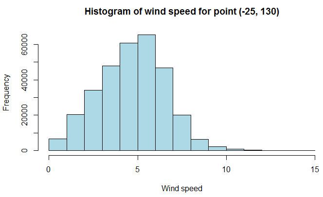
Histogram of wind speed for point (-25, 130) (latitude, longitude)

hist(result$ws, main = "Histogram of wind speed for point (-25, 130)", xlab = "Wind speed", col = "lightblue")

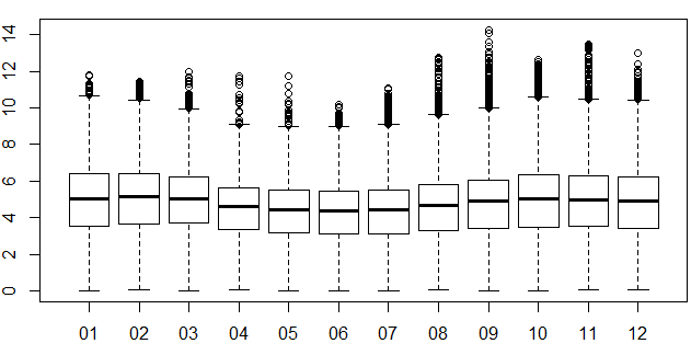
Monthly boxplot of wind speed

plot(as.factor(format(result$date, "%m")), result$ws)

OpenAIR package provides comprehensive tools to explore air pollution and wind data (see below).

library(openair)

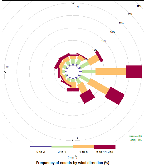
Wind rose shows the wind frequency from a particular direction. The data from the whole time interval are used

windRose(result)

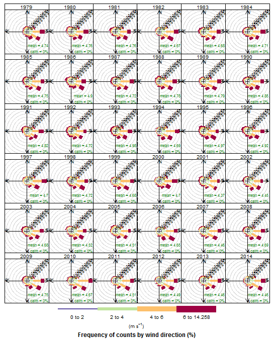
The same, but statistics is shown for each year separately

windRose(result, type = "year")

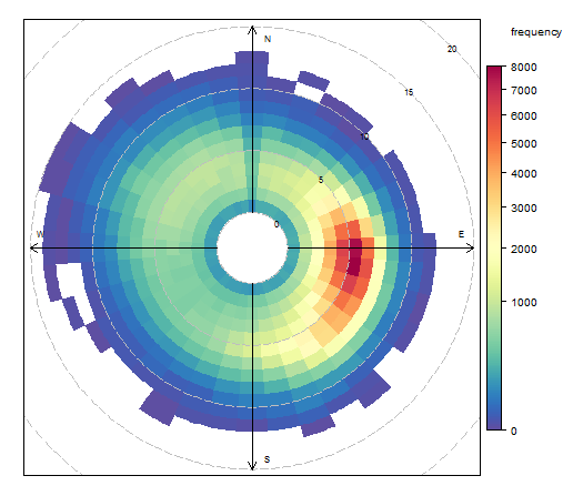
From OpenAir manual: “Each cell gives the total number of dates the wind was from that wind speed/direction. The number of dates is coded as a colour scale shown to the right. The scale itself is non-linear to help show the overall distribution.”

polarFreq(result)

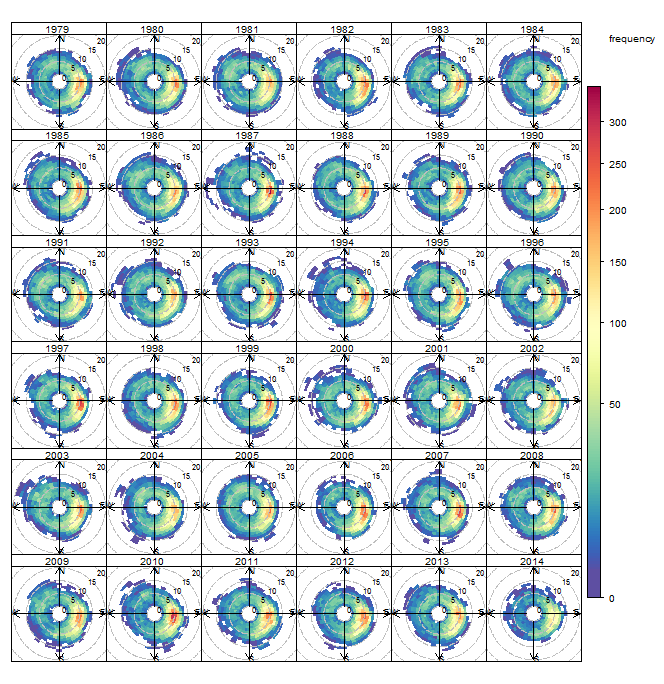
The same, but for a particular year

polarFreq(result, type = "year")

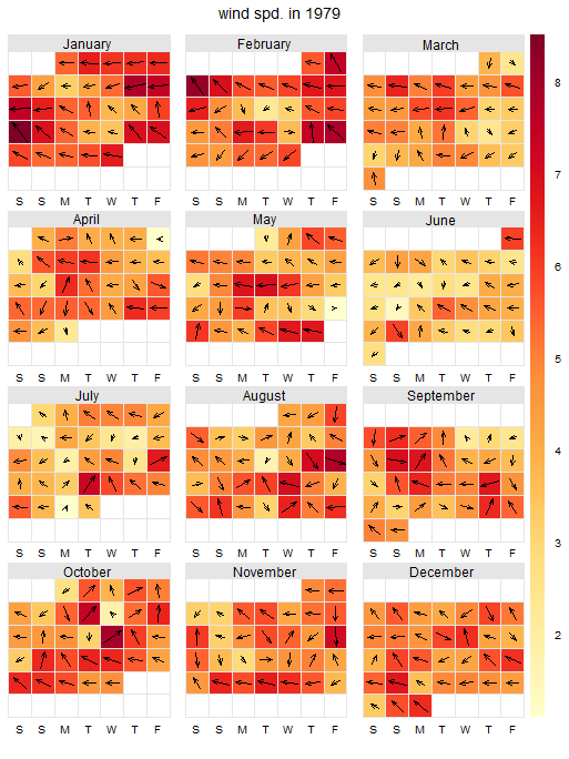
Display a calendar for a given year. In each cell of the calendar (each day) the wind direction is shown. The color of the cell is proportional to the wind speed. The longer the arrow, the greater wind speed is.

calendarPlot(result, pollutant = "ws", year = 1979, annotate = "ws")

If you would like to use the wind speed and direction data somewhere else, save it to CSV file.

fileName = "D:/Wind_speed_25_130.csv"   # Path to file
write.csv(file = fileName, x = result)

You can download the R code used in this tutorial with a single file [wpdm_file id=13]

Related links

• RWikience package download
• RWikience: introduction tutorial
• Tutorial on retrieving time series in Climate Wikience (without R)

Email

Facebook

Google

Linkedin

Twitter